AutoML Tables and the 'Chicago Taxi Trips' dataset
AutoML Tables was recently announced as a new member of GCP’s family of AutoML products. It lets you automatically build and deploy state-of-the-art machine learning models on structured data.
I thought it would be fun to try AutoML Tables on a dataset that’s been used for a number of recent TensorFlow-based examples: the ‘Chicago Taxi Trips’ dataset, which is one of a large number of public datasets hosted with BigQuery.
These examples use this dataset to build a neural net model (specifically, a “wide and deep” TensorFlow model) that predicts whether a given trip will result in a tip > 20%. (Many of these examples also show how to use the TensorFlow Extended (TFX) libraries for things like data validation, feature preprocessing, and model analysis).
We can’t directly compare the results of the following AutoML experimentation to those previous examples, since they’re using a different dataset and model architecture. However, we’ll use a roughly similar set of input features and stick to the spirit of these other examples by doing binary classification on the tip percentage.
In the rest of the blog post, we’ll walk through how to do that.
Step 1: Create a BigQuery table for the AutoML input dataset
AutoML Tables makes it easy to ingest data from BigQuery.
So, we’ll generate a version of the Chicago taxi trips public BigQuery table that has a new column reflecting whether or not the tip was > 20%. We’ll also do a bit of ‘bucketing’ of the lat/long information using the (new-ish and very cool) BigQuery GIS functions, and weed out rows where either the fare or trip miles are not > 0.
So, the first thing we’ll do is run a BigQuery query to generate this new version of the Chicago taxi dataset. Paste the following SQL into the BigQuery query window, or use this URL. Edit the SQL to use your own project and dataset prior to running the query.
Note: when I ran this query, it processed about 15.7 GB of data.
CREATE OR REPLACE TABLE `your-project.your-dataset.chicago_taxitrips_mod` AS (
WITH
  taxitrips AS (
  SELECT
    trip_start_timestamp,
    trip_end_timestamp,
    trip_seconds,
    trip_miles,
    pickup_census_tract,
    dropoff_census_tract,
    pickup_community_area,
    dropoff_community_area,
    fare,
    tolls,
    extras,
    trip_total,
    payment_type,
    company,
    pickup_longitude,
    pickup_latitude,
    dropoff_longitude,
    dropoff_latitude,
    IF((tips/fare >= 0.2),
      1,
      0) AS tip_bin
  FROM
    `bigquery-public-data.chicago_taxi_trips.taxi_trips`
  WHERE
    trip_miles > 0
    AND fare > 0)
SELECT
  trip_start_timestamp,
  trip_end_timestamp,
  trip_seconds,
  trip_miles,
  pickup_census_tract,
  dropoff_census_tract,
  pickup_community_area,
  dropoff_community_area,
  fare,
  tolls,
  extras,
  trip_total,
  payment_type,
  company,
  tip_bin,
  ST_AsText(ST_SnapToGrid(ST_GeogPoint(pickup_longitude,
        pickup_latitude), 0.1)) AS pickup_grid,
  ST_AsText(ST_SnapToGrid(ST_GeogPoint(dropoff_longitude,
        dropoff_latitude), 0.1)) AS dropoff_grid,
  ST_Distance(ST_GeogPoint(pickup_longitude,
      pickup_latitude),
    ST_GeogPoint(dropoff_longitude,
      dropoff_latitude)) AS euclidean,
  CONCAT(ST_AsText(ST_SnapToGrid(ST_GeogPoint(pickup_longitude,
          pickup_latitude), 0.1)), ST_AsText(ST_SnapToGrid(ST_GeogPoint(dropoff_longitude,
          dropoff_latitude), 0.1))) AS loc_cross
FROM
  taxitrips
LIMIT
  100000000
  )
You can see the use of the ST_SnapToGrid function to “bucket” the lat/long data, including a ‘cross’ of pickup with dropoff. We’re converting those fields to text and will treat them categorically. We’re also generating a new euclidean distance measure between pickup and dropoff using the ST_Distance function, and a feature cross of the pickup and dropoff grids.
Note: I also experimented with including the actual pickup and dropoff lat/lng values in the new table in addition to the derived grid values, but (unsurprisngly, since it can be hard for a NN to learn relationships between features) these additional inputs did not improve accuracy.
Step 2: Import your new table as an AutoML dataset
Then, return to the AutoML panel in the Cloud Console, and import your table —the new one in your own project that you created when running the query above — as a new AutoML Tables dataset.
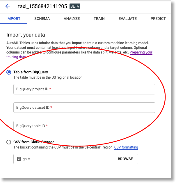
Import your new BigQuery table to create a new AutoML Tables dataset.
Step 3: Specify a schema, and launch the AutoML model training job
After the import has completed, you’ll next specify a schema for your dataset. Here is where you indicate which column is your ‘target’ (what you’d like to learn to predict), as well as the column types.
We’ll use the tip_bin column as the target. Recall that this is one of the new columns we created when generating the new BigQuery table. So, the ML task will be to learn how to predict — given other information about the trip — whether or not the tip will be over 20%.
Note that once you select this column as the target, AutoML automatically suggests that it should build a classification model, which is what we want.
Then, we’ll adjust some of the column types. AutoML does a pretty good job of inferring what they should be, based on the characteristics of the dataset. However, we’ll set the ‘census tract’ and ‘community area’ columns (for both pickup and dropoff) to be treated as categorical, not numerical. We’ll also set the the pickup_grid,
dropoff_grid, and loc_cross columns as categorical.
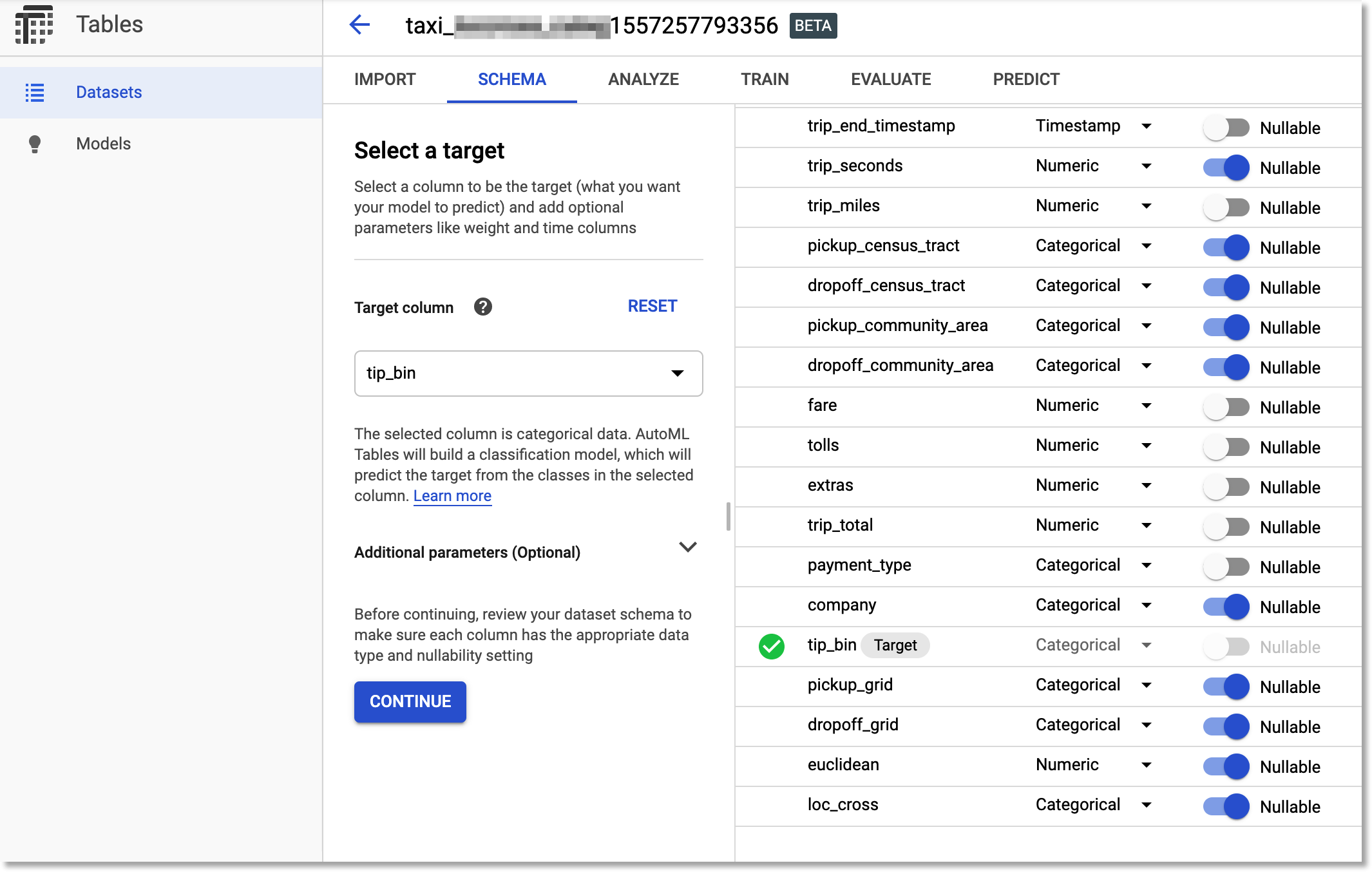
Specify the input schema for your training job.
We can view an analysis of the dataset as well. Some rows have a lot of missing fields. We won’t take any further action for this example, but if this was your own dataset, this might indicate places where your data collection process was problematic or where your daataset needed some cleanup. You can also check the number of distinct values for a column, and look at the correlation of a column with the target. (Note that the tolls field has low correlation with the target).
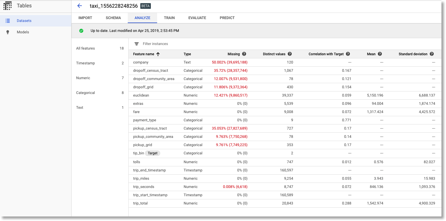
AutoML Table's analysis of the dataset.
Now we’re ready to kick off the training job. We need to tell it how many node-hours to spend. Here I’m using 3, but you might want to use just 1 hour in your experiment. (Here’s the (beta) pricing guide.)
We’ll also tell AutoML which (non-target) columns to use as input. Here, we’ll indicate to drop
the trip_total. This value tracks with tip, so for the purposes of this experiment, its inclusion is ‘cheating’. We’ll also tell it to drop the tolls field, which the analysis indicated had very low correlation with the target.
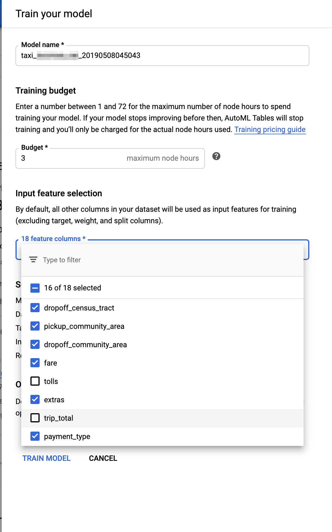
Setting up an AutoML Tables training job.
Evaluating the AutoML model
When the training completes, you’ll get an email notification. AutoML automatically generates and displays model evaluation metrics for you. We can see, for example, that for this training run, model accuracy is 90.6% and the AUC ROC is 0.954. (Your results will probably vary a bit).
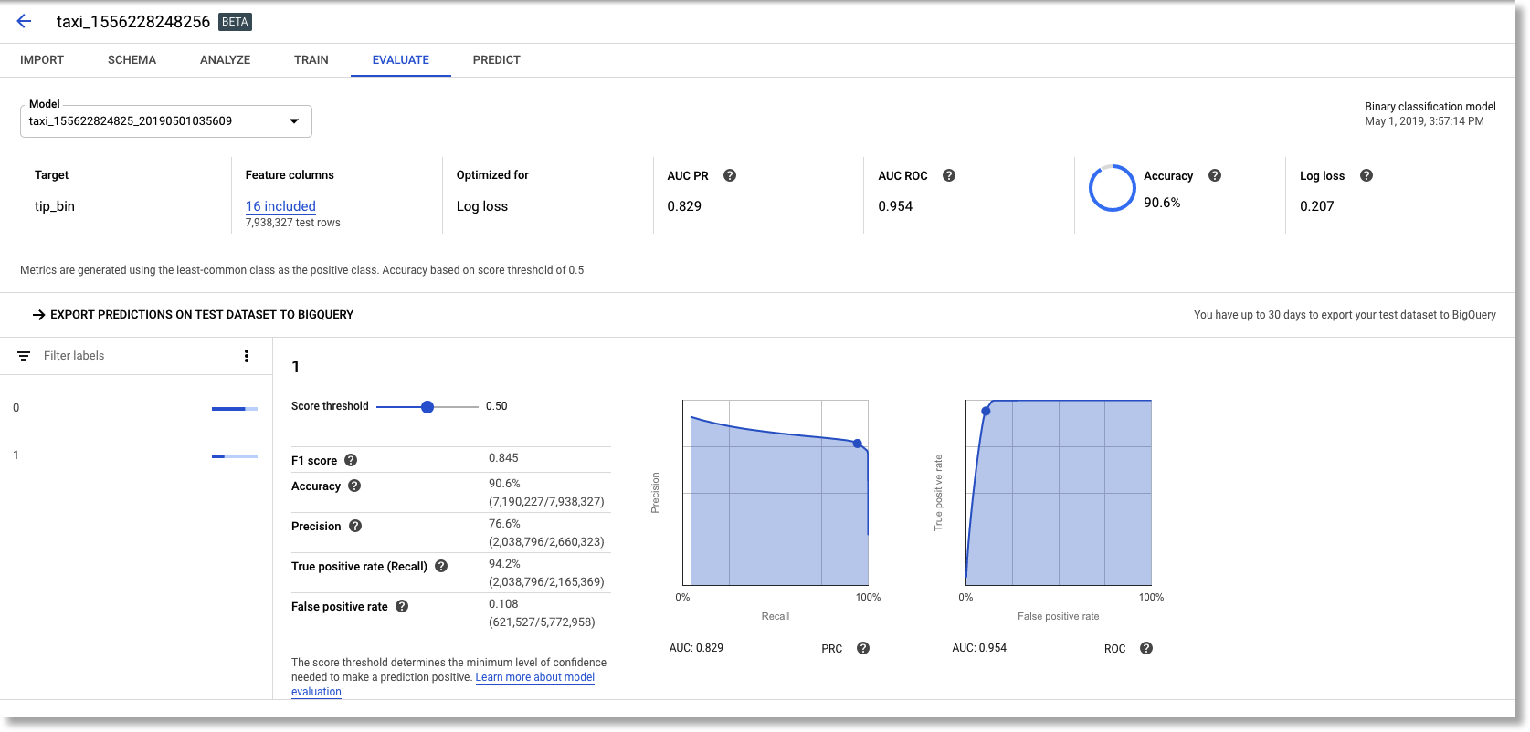
AutoML Tables model evaluation info.
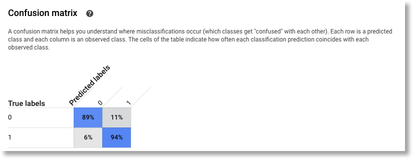
It also generates a confusion matrix…
…and a histogram of the input features that were of most importance. This histogram is kind of interesting: it suggests that payment_type was most important. (My guess: people are more likely to tip if they’re putting the fare on a credit card, where a tip is automatically suggested; and cash tips tend to be underreported). It looks like the pickup and dropoff info was not that informative, though information about trip distance, and the pickup/dropoff cross, were a bit more so.
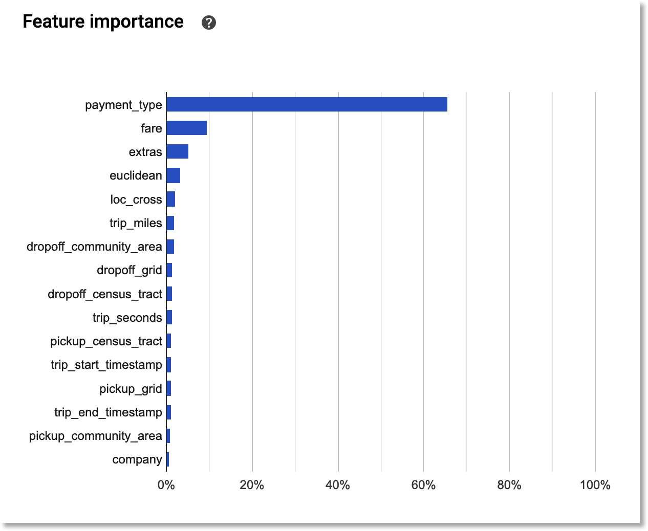
The most important features in the dataset, for predicting the given target.
View your evaluation results in BigQuery
You can also export your evaluation results to a new BigQuery table, which lets you see the predicted score and label for the test dataset instances.
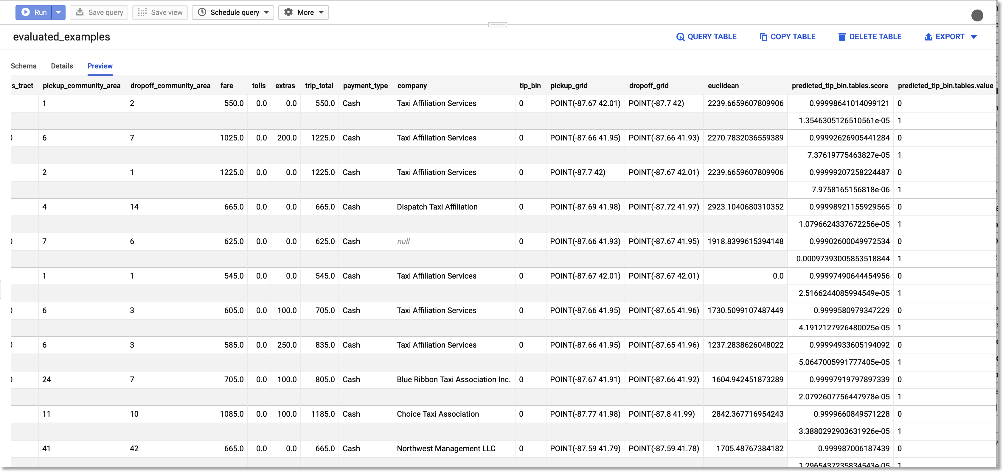
Export your model evaluation results to BigQuery.
Step 4: Use your new model for prediction
Once you’ve trained your model, you can use it for prediction. You can opt to use a BigQuery table or Google Cloud Storage (GCS) files for both input sources and outputs.
You can also perform online prediction. For this, you’ll first need to deploy your model. This process will take a few minutes.
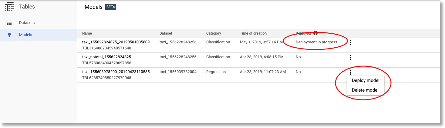
You can deploy (or delete) any of your trained models.
Once deployment’s done, you can send real-time REST requests to the AutoML Tables API. The AutoML web UI makes it easy to experiment with this API. (See the pricing guide— if you’re just experimenting, you may want to take down your deployed model once you’re done.)
Note the linked “getting started” instructions on creating a service account first.
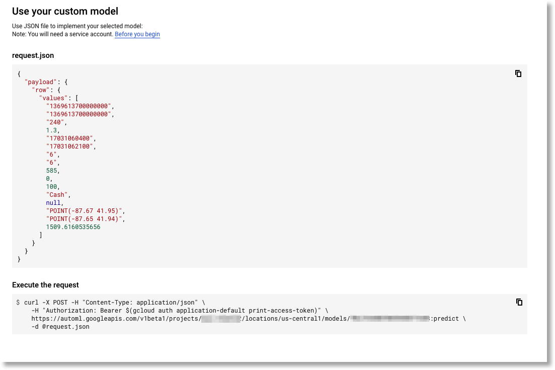
Experiment with using the online prediction REST API from the AutoML UI.
You’ll see json-formatted responses similar to this one:
{
  "payload": [
    {
      "tables": {
        "score": 0.999618,
        "value": "0"
      }
    },
    {
      "tables": {
        "score": 0.0003819269,
        "value": "1"
      }
    }
  ]
}
Wrap-up
In this post, I showed how straightforward it is to use AutoML Tables to train, evaluate, and use state-of-the-art deep neural net models that are based on your own structured data, but without needing to build model code or manage distributed training; and then deploy the result for scalable serving.
The example also showed how easy it is to leverage BigQuery queries (in particular I highlighted some of the the BigQuery GIS functions) to do some feature pre-processing.