Training an AutoML Tables model with BigQuery ML
How to use BigQuery ML to train an AutoML Tables model
- Introduction
- About the dataset and modeling task
- Specifying training, eval, and test datasets
- Tables schema configuration and BQML
- Training the AutoML Tables model via BQML
- Evaluating your trained custom model
- Using your BQML AutoML Tables model for prediction
- Summary
Introduction
BigQuery ML (BQML) enables users to create and execute machine learning models in BigQuery by using SQL queries.
AutoML Tables lets you automatically build, analyze, and deploy state-of-the-art machine learning models using your own structured data, and explain prediction results. It’s useful for a wide range of machine learning tasks, such as asset valuations, fraud detection, credit risk analysis, customer retention prediction, analyzing item layouts in stores, solving comment section spam problems, quickly categorizing audio content, predicting rental demand, and more. (This blog post gives more detail on many of its capabilities).
Recently, BQML added support for AutoML Tables models (in Beta). This makes it easy to train Tables models on your BigQuery data using standard SQL, directly from the BigQuery UI (or API), and to evaluate and use the models for prediction directly via SQL as well.
In this post, we’ll take a look at how to do this, and show a few tips as well.
About the dataset and modeling task
The Cloud Public Datasets Program makes available public datasets that are useful for experimenting with machine learning. We’ll use data that is essentially a join of two public datasets stored in BigQuery: London Bike rentals and NOAA weather data, with some additional processing to clean up outliers and derive additional GIS and day-of-week fields. The table we’ll use is here: aju-dev-demos.london_bikes_weather.bikes_weather.
Using this dataset, we’ll build a regression model to predict the duration of a bike rental based on information about the start and end rental stations, the day of the week, the weather on that day, and other data. (If we were running a bike rental company, we could use these predictions—and their explanations—to help us anticipate demand and even plan how to stock each location).
Specifying training, eval, and test datasets
AutoML Tables will split the data you send it into its own training/test/validation sets.
Note: it’s also possible to specify the data split column as a BQML model creation option:
DATA_SPLIT_COL = string_value.string_valueis one of the columns in the training data and should be either a timestamp or string column. See the documentation for more detail.
For BQML, we’ll split the data into a set to use for the training process, and reserve a ‘test’ dataset that AutoML training never sees. We don’t want to just grab a sequential slice of the table for each. There’s an easy way to accomplish this in a repeatable manner by using the Farm Hash algorithm, implemented as the FARM_FINGERPRINT BigQuery SQL function. We’d like to create a 90/10 split.
So, the query to generate training data will include a clause like this:
WHERE ABS(MOD(FARM_FINGERPRINT(timestamp), 10)) < 9
Similarly, the query to generate the ‘test’ set will use this clause:
WHERE ABS(MOD(FARM_FINGERPRINT(timestamp), 10)) = 9
Using this approach, we can build SELECT clauses with reproducible results that give us datasets with the split proportions we want.
Tables schema configuration and BQML
If you’ve used AutoML Tables, you may have noticed that after a dataset is ingested, it’s possible to adjust the inferred field (column) schema information. For example, you might have some fields with numeric values that you’d like to treat as categorical when you train your custom model. This is the case for our dataset, where we’d like to treat the numeric rental station IDs as categorical.
With BQML, it’s not currently possible to explicitly specify the schema for the model inputs, but for numerics that we want to treat as categorical, we can provide a strong hint by casting them to strings; then Tables will decide whether to treat such values as ‘text’ or ‘categorical’. So, in the SQL below, you’ll see that the day_of_week, start_station_id, and end_station_id columns are all cast to strings.
Training the AutoML Tables model via BQML
To train the Tables model, we’ll pick the AUTOML_REGRESSOR model type (since we want to predict duration, a numeric value. In the query, we’ll specify duration in the input_label_cols list (thus indicating the “label” column”, and set budget_hours to 1, meaning that we’re budgeting one hour of training time. (The training process, which includes setup and teardown, etc., will typically take longer).
Here’s the resultant BigQuery query (to run it yourself, substitute your project id, dataset, and model name in the first line, then paste the query into the BigQuery UI query window in the Cloud Console):
CREATE OR REPLACE MODEL `YOUR-PROJECT-ID.YOUR-DATASET.YOUR-MODEL-NAME`
       OPTIONS(model_type='AUTOML_REGRESSOR',
               input_label_cols=['duration'],
               budget_hours=1.0)
AS SELECT
  duration, ts, cast(day_of_week as STRING) as dow, start_latitude, start_longitude, end_latitude,
  end_longitude, euclidean, loc_cross, prcp, max, min, temp, dewp,
  cast(start_station_id as STRING) as ssid, cast(end_station_id as STRING) as esid
FROM `aju-dev-demos.london_bikes_weather.bikes_weather`
WHERE
ABS(MOD(FARM_FINGERPRINT(cast(ts as STRING)), 10)) < 9
Note the casts to STRING and the use of FARM_FINGERPRINT as discussed above.
(If you’ve taken a look at the bikes_weather table, you might notice that the SELECT clause does not include the bike_id column. A previously-run AutoML Tables analysis of the global feature importance of the dataset fields indicated that bike_id had negligible impact, so we won’t use it for this model).
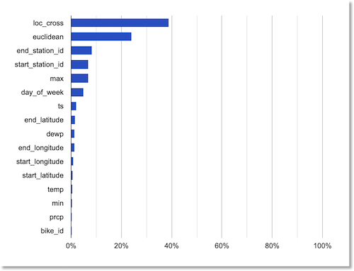
Global feature importance rankings.
Evaluating your trained custom model
After the training has completed, you can view the evaluation metrics for your custom model, and also run your own evaluation query yourself. You can view the evaluation metrics generated during the training process by clicking on the model name in the BigQuery UI, then click on the “Evaluation” tab in the central panel. It will look something like this:
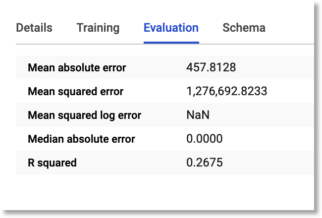
Model evaluation metrics generated during the training process
(At time of writing, some of this data is incomplete, but that will change soon).
The BigQuery SQL to run your own evaluation query for the trained model looks like this (again, substitute your own project, dataset, and model name):
SELECT
  *
FROM
  ML.EVALUATE(MODEL `YOUR-PROJECT-ID.YOUR-DATASET.YOUR-MODEL-NAME`, (
SELECT
  duration, ts, cast(day_of_week as STRING) as dow, start_latitude, start_longitude, end_latitude,
  end_longitude, euclidean, loc_cross, prcp, max, min, temp, dewp,
  cast(start_station_id as STRING) as ssid, cast(end_station_id as STRING) as esid
FROM
  `aju-dev-demos.london_bikes_weather.bikes_weather`
WHERE
 ABS(MOD(FARM_FINGERPRINT(cast(ts as STRING)), 10)) = 9
 ))
Note that via the FARM_FINGERPRINT function, we’re using a different dataset for evaluation than we used for training.
The evaluation results should look something like the following. The metrics will be a bit different from those above, since we’re using different data than AutoML Tables used for its eval split.
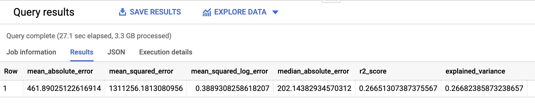
Model evaluation results.
Did our schema hints help?
It’s interesting to check whether the schema hints (casting some of the numeric fields to strings) made a difference in model accuracy.
To try this yourself, create another differently-named model as shown in the training section above, but for the SELECT clause, don’t include the casts to STRING, e.g.:
...AS SELECT
  duration, ts, day_of_week, start_latitude, start_longitude, end_latitude,
  end_longitude, euclidean, loc_cross, prcp, max, min, temp, dewp, start_station_id, end_station_id
Then, evaluate this second model (again substituting the details for your own project):
SELECT
  *
FROM
  ML.EVALUATE(MODEL `YOUR-PROJECT-ID.YOUR-DATASET.YOUR-MODEL-NAME2`, (
SELECT
  duration, ts, day_of_week, start_latitude, start_longitude, end_latitude,
  end_longitude, euclidean, loc_cross, prcp, max, min, temp, dewp, start_station_id, end_station_id
FROM
  `aju-dev-demos.london_bikes_weather.bikes_weather`
WHERE
 ABS(MOD(FARM_FINGERPRINT(cast(ts as STRING)), 10)) = 9
 ))
When I evaluated this second model, which kept the station IDs and day of week as numerics, the results showed that this model was somewhat less accurate:
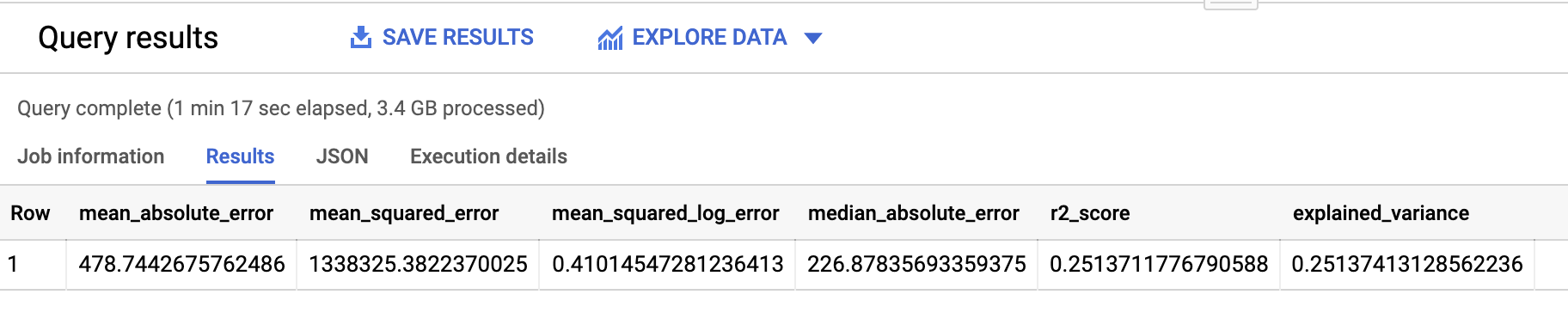
Evaluation results for the model that did not cast categorical numerics to strings.
Using your BQML AutoML Tables model for prediction
Once your model is trained, and you’ve ascertained it’s accurate enough, you can use it for prediction.
Here’s an example of how to do that. Via the FARM_FINGERPRINT function, we’re drawing from our “test” split, but because the resultant dataset is large, we’re just grabbing a few rows (200) for the query below:
SELECT * FROM ML.PREDICT(MODEL `YOUR-PROJECT-ID.YOUR-DATASET.YOUR-MODEL-NAME`,
(SELECT   duration, ts, cast(day_of_week as STRING) as dow, start_latitude, start_longitude, end_latitude,
  end_longitude, euclidean, loc_cross, prcp, max, min, temp, dewp,
  cast(start_station_id as STRING) as ssid, cast(end_station_id as STRING) as esid
 FROM `aju-dev-demos.london_bikes_weather.bikes_weather`
 WHERE ABS(MOD(FARM_FINGERPRINT(cast(ts as STRING)), 10)) = 9)) limit 200
The prediction results will look something like this (click to see larger version):
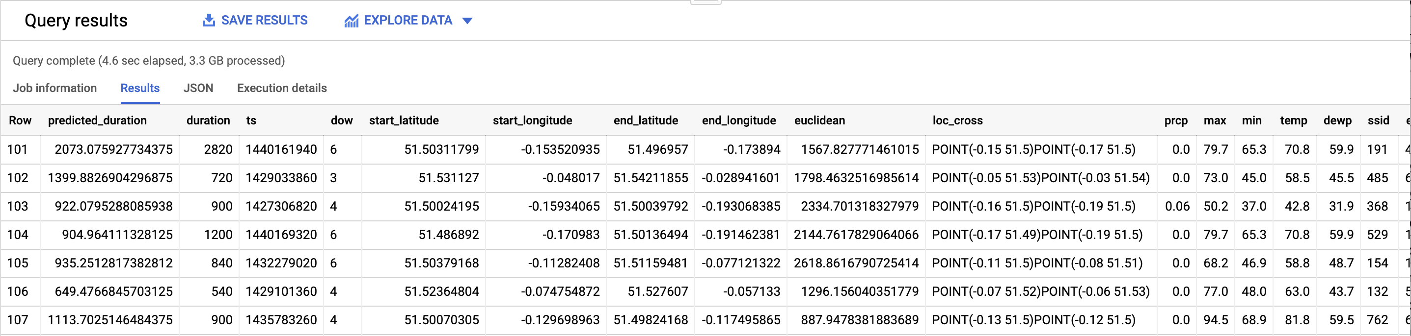
Model prediction results.
Note that while the query above is “standalone”, you can of course access model prediction results as part of a larger BigQuery query too.
Summary
In this post, we showed how to train an AutoML Tables model using BQML, evaluate the model, and then use it for prediction— all from BigQuery. The BQML documentation has more detail on getting started, and resources for the other model types available through BQML.