Creating an AutoML Tables end-to-end workflow on Cloud AI Platform Pipelines
An overview of new AutoML Tables features, via a Cloud AI Platform Pipelines example showing an end-to-end workflow
- Introduction
- Using Cloud AI Platform Pipelines or Kubeflow Pipelines to orchestrate a Tables workflow
- The steps executed by the pipeline
- Getting explanations about your model’s predictions
- The AutoML Tables UI in the Cloud Console
- Export the trained model and serve it on a GKE cluster
- A deeper dive into the pipeline code
Introduction
AutoML Tables lets you automatically build, analyze, and deploy state-of-the-art machine learning models using your own structured data.
A number of new AutoML Tables features have been released recently. These include:
- An improved Python client library
- The ability to obtain explanations for your online predictions
- The ability to export your model and serve it in a container anywhere
- The ability to view model search progress and final model hyperparameters in Cloud Logging
This post gives a tour of some of these new features via a Cloud AI Platform Pipelines example, that shows end-to-end management of an AutoML Tables workflow.
The example pipeline creates a dataset, imports data into the dataset from a BigQuery view, and trains a custom model on that data. Then, it fetches evaluation and metrics information about the trained model, and based on specified criteria about model quality, uses that information to automatically determine whether to deploy the model for online prediction. Once the model is deployed, you can make prediction requests, and optionally obtain prediction explanations as well as the prediction result. In addition, the example shows how to scalably serve your exported trained model from your Cloud AI Platform Pipelines installation for prediction requests.
You can manage all the parts of this workflow from the Tables UI as well, or programmatically via a notebook or script. But specifying this process as a workflow has some advantages: the workflow becomes reliable and repeatable, and Pipelines makes it easy to monitor the results and schedule recurring runs. For example, if your dataset is updated regularly—say once a day— you could schedule a workflow to run daily, each day building a model that trains on an updated dataset. (With a bit more work, you could also set up event-based triggering pipeline runs, for example when new data is added to a Google Cloud Storage bucket.)
About the example dataset and scenario
The Cloud Public Datasets Program makes available public datasets that are useful for experimenting with machine learning. For our examples, we’ll use data that is essentially a join of two public datasets stored in BigQuery: London Bike rentals and NOAA weather data, with some additional processing to clean up outliers and derive additional GIS and day-of-week fields. Using this dataset, we’ll build a regression model to predict the duration of a bike rental based on information about the start and end rental stations, the day of the week, the weather on that day, and other data. If we were running a bike rental company, we could use these predictions—and their explanations—to help us anticipate demand and even plan how to stock each location. While we’re using bike and weather data here, you can use AutoML Tables for tasks as varied as asset valuations, fraud detection, credit risk analysis, customer retention prediction, analyzing item layouts in stores, and many more.
Using Cloud AI Platform Pipelines or Kubeflow Pipelines to orchestrate a Tables workflow
You can run this example via a Cloud AI Platform Pipelines installation, or via Kubeflow Pipelines on a Kubeflow on GKE installation. Cloud AI Platform Pipelines was recently launched in Beta. Slightly different variants of the pipeline specification are required depending upon which you’re using. (It would be possible to run the example on other Kubeflow installations too, but that would require additional credentials setup not covered in this tutorial).
Install a Cloud AI Platform Pipelines cluster
You can create an AI Platform Pipelines installation with a few clicks. Access AI Platform Pipelines by visiting the AI Platform Panel in the Cloud Console.
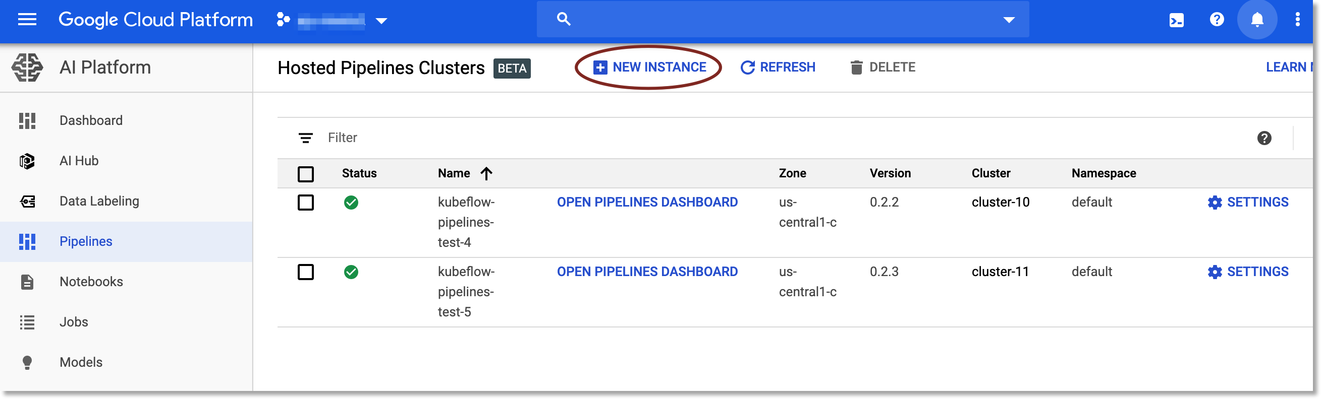
Create a new Pipelines instance.
See the documentation for more detail.
(You can also do this installation from the command line onto an existing GKE cluster if you prefer. If you do, for consistency with the UI installation, create the GKE cluster with --scopes cloud-platform).
Or, install Kubeflow to use Kubeflow Pipelines
You can also run this example from a Kubeflow installation. For the example to work out of the box, you’ll need a Kubeflow on GKE installation, set up to use IAP. An easy way to do this is via the Kubeflow ‘click to deploy’ web app, or you can follow the command-line instructions here.
Upload and run the Tables end-to-end Pipeline
Once a Pipelines installation is running, we can upload the example AutoML Tables pipeline. Click on Pipelines in the left nav bar of the Pipelines Dashboard. Click on Upload Pipeline.
- For Cloud AI Platform Pipelines, upload
tables_pipeline_caip.py.tar.gz. This archive points to the compiled version of this pipeline, specified and compiled using the Kubeflow Pipelines SDK. - For Kubeflow Pipelines on a Kubeflow installation, upload
tables_pipeline_kf.py.tar.gz. This archive points to the compiled version of this pipeline. To run this example on a KF installation, you will need to give the<deployment-name>-user@<project-id>.iam.gserviceaccount.comservice accountAutoML Adminprivileges.
Note: The difference between the two pipelines relates to how GCP authentication is handled. For the Kubeflow pipeline, we’ve added
.apply(gcp.use_gcp_secret('user-gcp-sa'))annotations to the pipeline steps. This tells the pipeline to use the mounted secret—set up during the installation process— that provides GCP account credentials. With the Cloud AI Platform Pipelines installation, the GKE cluster nodes have been set up to use thecloud-platformscope. With recent Kubeflow releases, use of the mounted secret is no longer necessary, but we include both versions for compatibility.
The uploaded pipeline graph will look similar to this:
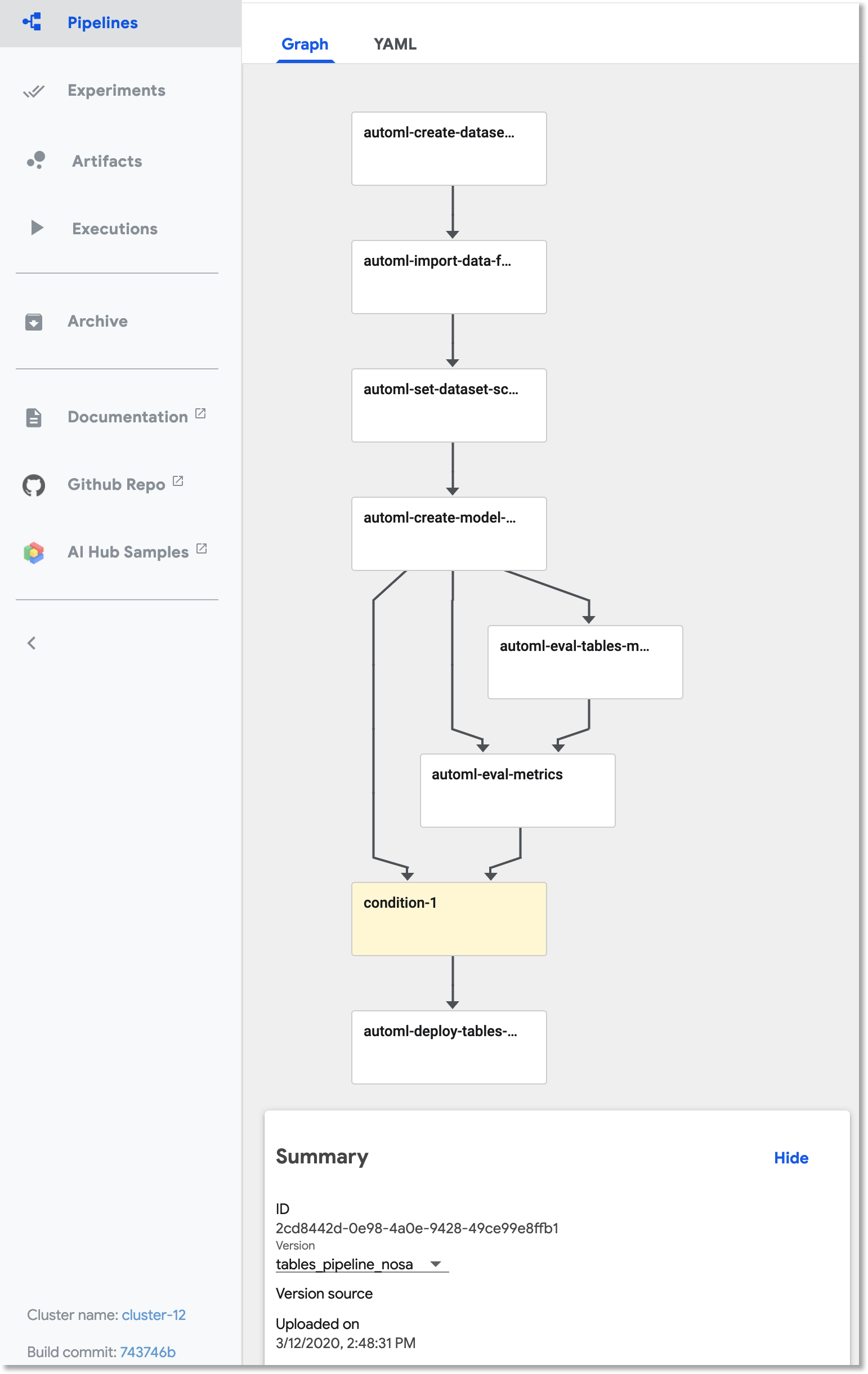
The uploaded Tables 'end-to-end' pipeline.
Click the +Create Run button to run the pipeline. You will need to fill in some pipeline parameters.
Specifically, replace YOUR_PROJECT_HERE with the name of your project; replace YOUR_DATASET_NAME with the name you want to give your new dataset (make it unique, and use letters, numbers and underscores up to 32 characters); and replace YOUR_BUCKET_NAME with the name of a GCS bucket. Do not include the gs:// prefix— just enter the name. This bucket should be in the same region as that specified by the gcp_region parameter. E.g., if you keep the default us-central1 region, your bucket should also be a regional (not multi-regional) bucket in the us-central1 region. ++double check that this is necessary.++
If you want to schedule a recurrent set of runs, you can do that instead. If your data is in BigQuery— as is the case for this example pipeline— and has a temporal aspect, you could define a view to reflect that, e.g. to return data from a window over the last N days or hours. Then, the AutoML pipeline could specify ingestion of data from that view, grabbing an updated data window each time the pipeline is run, and building a new model based on that updated window.
The steps executed by the pipeline
The example pipeline creates a dataset, imports data into the dataset from a BigQuery view, and trains a custom model on that data. Then, it fetches evaluation and metrics information about the trained model, and based on specified criteria about model quality, uses that information to automatically determine whether to deploy the model for online prediction. We’ll take a closer look at each of the pipeline steps, and how they’re implemented.
Create a Tables dataset and adjust its schema
This pipeline creates a new Tables dataset, and ingests data from a BigQuery table for the “bikes and weather” dataset described above. These actions are implemented by the first two steps in the pipeline (the automl-create-dataset-for-tables and automl-import-data-for-tables steps).
While we’re not showing it in this example, AutoML Tables supports ingestion from BigQuery views as well as tables. This can be an easy way to do feature engineering: leverage BigQuery’s rich set of functions and operators to clean and transform your data before you ingest it.
When the data is ingested, AutoML Tables infers the data type for each field (column). In some cases, those inferred types may not be what you want. For example, for our “bikes and weather” dataset, several ID fields (like the rental station IDs) are set by default to be numeric, but we want them treated as categorical when we train our model. In addition, we want to treat the loc_cross strings as categorical rather than text.
We make these adjustments programmatically, by defining a pipeline parameter that specifies the schema changes we want to make. Then, in the automl-set-dataset-schema pipeline step, for each indicated schema adjustment, we call update_column_spec:
client.update_column_spec(
          dataset_display_name=dataset_display_name,
          column_spec_display_name=column_spec_display_name,
          type_code=type_code,
          nullable=nullable
      )
Before we can train the model, we also need to specify the target column— what we want our model to predict. In this case, we’ll train the model to predict rental duration. This is a numeric value, so we’ll be training a regression model.
client.set_target_column(
              dataset_display_name=dataset_display_name,
              column_spec_display_name=target_column_spec_name
          )
Train a custom model on the dataset
Once the dataset is defined and its schema set properly, the pipeline will train the model. This happens in the automl-create-model-for-tables pipeline step. Via pipeline parameters, we can specify the training budget, the optimization objective (if not using the default), and can additionally specify which columns to include or exclude from the model inputs.
You may want to specify a non-default optimization objective depending upon the characteristics of your dataset. This table describes the available optimization objectives and when you might want to use them. For example, if you were training a classification model using an imbalanced dataset, you might want to specify use of AUC PR (MAXIMIZE_AU_PRC), which optimizes results for predictions for the less common class.
client.create_model(
    model_display_name,
    train_budget_milli_node_hours=train_budget_milli_node_hours,
    dataset_display_name=dataset_display_name,
    optimization_objective=optimization_objective,
    include_column_spec_names=include_column_spec_names,
    exclude_column_spec_names=exclude_column_spec_names,
  )
View model search information via Cloud Logging
You can view details about an AutoML Tables model via Cloud Logging. Using Logging, you can see the final model hyperparameters as well as the hyperparameters and object values used during model training and tuning.
An easy way to access these logs is to go to the AutoML Tables page in the Cloud Console. Select the Models tab in the left navigation pane and click on the model you’re interested in. Click the “Model” link to see the final hyperparameter logs. To see the tuning trial hyperparameters, click the “Trials” link.
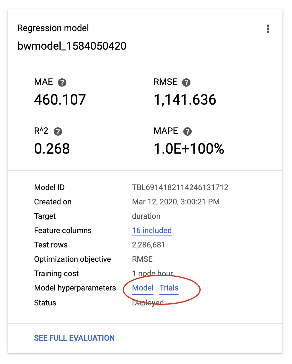
View a model's search logs from its evaluation information.
For example, here is a look at the Trials logs a custom model trained on the “bikes and weather” dataset, with one of the entries expanded in the logs:
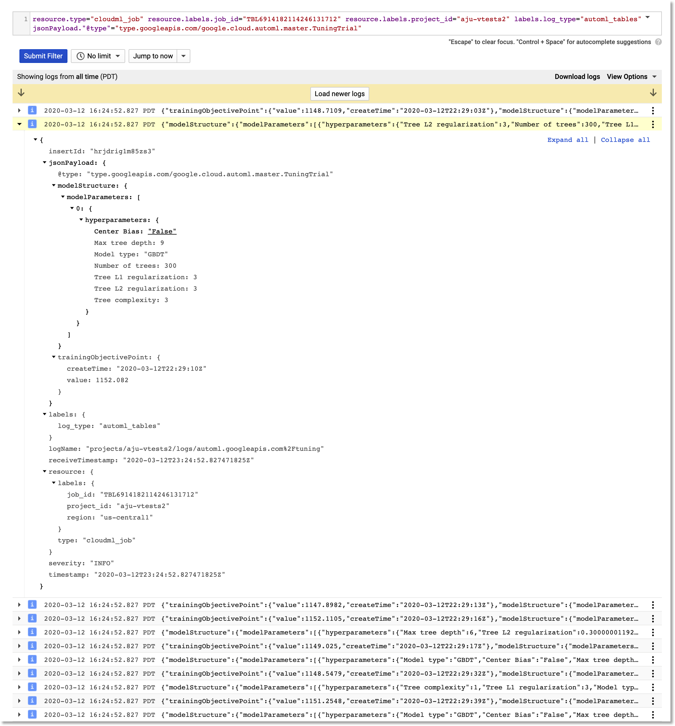
The 'Trials' logs for a "bikes and weather" model
Custom model evaluation
Once your custom model has finished training, the pipeline moves on to its next step: model evaluation. We can access evaluation metrics via the API. We’ll use this information to decide whether or not to deploy the model.
These actions are factored into two steps. The process of fetching the evaluation information can be a general-purpose component (pipeline step) used in many situations; and then we’ll follow that with a more special-purpose step, that analyzes that information and uses it to decide whether or not to deploy the trained model.
In the first of these pipeline steps— the automl-eval-tables-model step— we’ll retrieve the evaluation and global feature importance information.
model = client.get_model(model_display_name=model_display_name)
feat_list = [(column.feature_importance, column.column_display_name)
        for column in model.tables_model_metadata.tables_model_column_info]
evals = list(client.list_model_evaluations(model_display_name=model_display_name))
AutoML Tables automatically computes global feature importance for a trained model. This shows, across the evaluation set, the average absolute attribution each feature receives. Higher values mean the feature generally has greater influence on the model’s predictions. This information is useful for debugging and improving your model. If a feature’s contribution is negligible—if it has a low value—you can simplify the model by excluding it from future training. The pipeline step renders the global feature importance data as part of the pipeline run’s output:
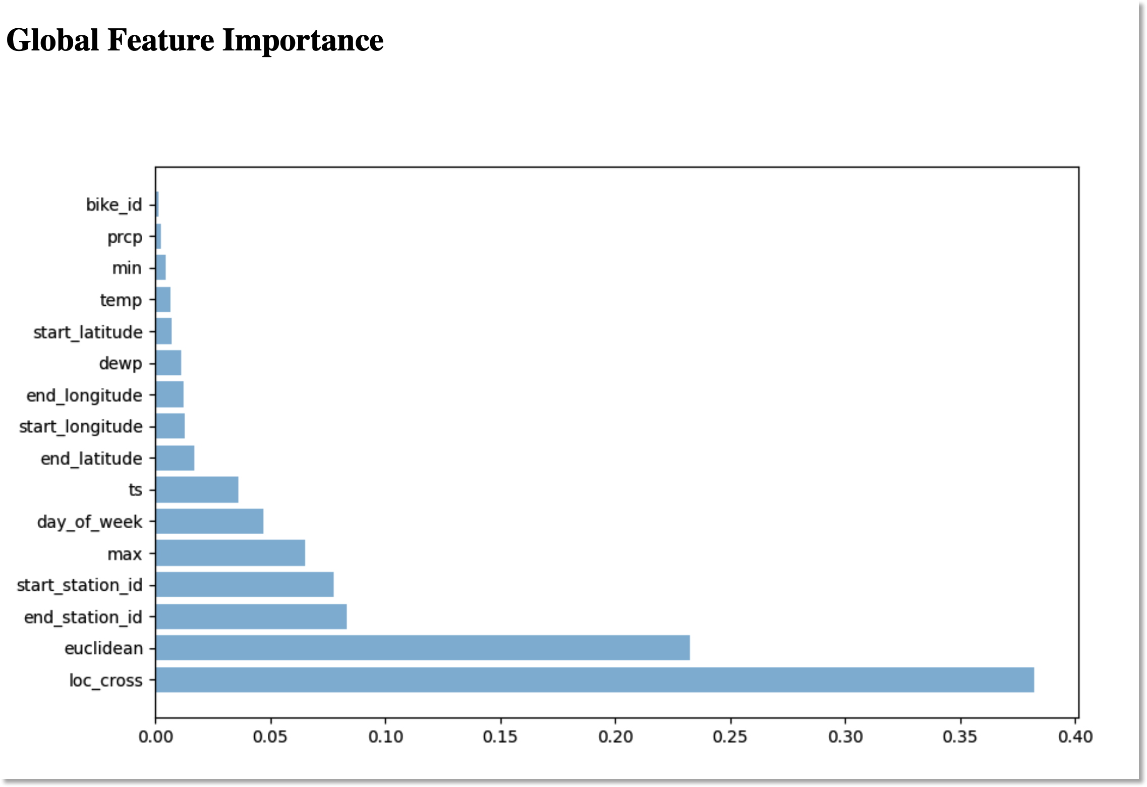
Global feature importance for the model inputs, rendered by a Kubeflow Pipeline step.
For our example, based on the graphic above, we might try training a model without including bike_id.
In the following pipeline step— the automl-eval-metrics step— the evaluation output from the previous step is grabbed as input, and parsed to extract metrics that we’ll use in conjunction with pipeline parameters to decide whether or not to deploy the model. Note that this component is more special-purpose: unlike the other components in this pipeline, which support generalizable operations, this component— while it is parameterized— is specific in how it analyzes the evaluation info and decides whether or not to do the deployment.
One of the pipeline input parameters allows specification of metric thresholds. In this example, we’re training a regression model, and we’re specifying a mean_absolute_error (MAE) value as a threshold in the pipeline input parameters:
{"mean_absolute_error": 450}
The automl-eval-metrics pipeline step compares the model evaluation information to the given threshold constraints. In this case, if the MAE is < 450, the model will not be deployed. The pipeline step outputs that decision, and displays the evaluation information it’s using as part of the pipeline run’s output:
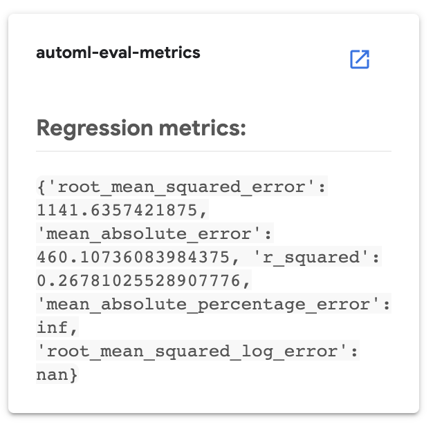
Information about a model's evaluation, rendered by a Kubeflow Pipeline step.
(Conditional) model deployment
You can deploy any of your custom Tables models to make them accessible for online prediction requests. The pipeline code uses a conditional test to determine whether or not to run the step that deploys the model, based on the output of the evaluation step described above:
with dsl.Condition(eval_metrics.outputs['deploy'] == True):
  deploy_model = deploy_model_op( ... )
Only if the model meets the given criteria, will the deployment step (called automl-deploy-tables-model) be run, and the model be deployed automatically as part of the pipeline run:
response = client.deploy_model(model_display_name=model_display_name)
You can always deploy a model later if you like.
Putting it together: The full pipeline execution
The figure below shows the result of a pipeline run. In this case, the conditional step was executed— based on the model evaluation metrics— and the trained model was deployed. Via the UI, you can view outputs, logs for each step, run artifacts and lineage information, and more. See this post for more detail.
++TODO: replace the following figure with something better++
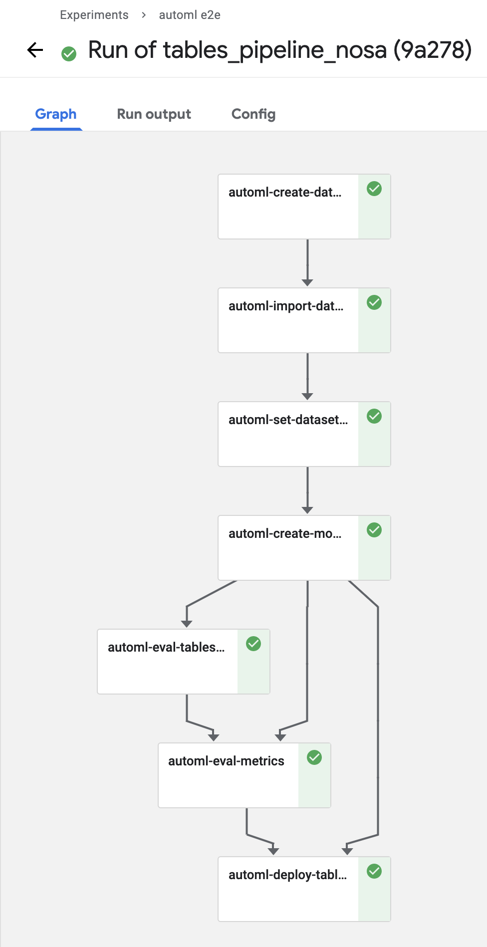
Execution of a pipeline run. You can view outputs, logs for each step, run artifacts and lineage information, and more.
Getting explanations about your model’s predictions
Once a model is deployed, you can request predictions from that model. You can additionally request explanations for local feature importance: a score showing how much (and in which direction) each feature influenced the prediction for a single example. See this blog post for more information on how those values are calculated.
Here is a notebook example of how to request a prediction and its explanation using the Python client libraries.
from google.cloud import automl_v1beta1 as automl
client = automl.TablesClient(project=PROJECT_ID, region=REGION)

response = client.predict(
    model_display_name=model_display_name,
    inputs=inputs,
    feature_importance=True,
)
The prediction response will have a structure like this. (The notebook above shows how to visualize the local feature importance results using matplotlib.)
It’s easy to explore local feature importance through the Cloud Console’s AutoML Tables UI as well. After you deploy a model, go to the TEST & USE tab of the Tables panel, select ONLINE PREDICTION, enter the field values for the prediction, and then check the Generate feature importance box at the bottom of the page. The result will show the feature importance values as well as the prediction. This blog post gives some examples of how these explanations can be used to find potential issues with your data or help you better understand your problem domain.
The AutoML Tables UI in the Cloud Console
With this example we’ve focused on how you can automate a Tables workflow using Kubeflow pipelines and the Python client libraries.
All of the pipeline steps can also be accomplished via the AutoML Tables UI in the Cloud Console, including many useful visualizations, and other functionality not implemented by this example pipeline— such as the ability to export the model’s test set and prediction results to BigQuery for further analysis.
Export the trained model and serve it on a GKE cluster
Recently, Tables launched a feature to let you export your full custom model, packaged so that you can serve it via a Docker container. (Under the hood, it is using TensorFlow Serving). This lets you serve your models anywhere that you can run a container, including a GKE cluster. This means that you can run a model serving service on your AI Platform Pipelines or Kubeflow installation, both of which run on GKE.
This blog post walks through the steps to serve the exported model (in this case, using Cloud Run). Follow the instructions in the post through the “View information about your exported model in TensorBoard” section. Here, we’ll diverge from the rest of the post and create a GKE service instead.
Make a copy of deploy_model_for_tables/model_serve_template.yaml file and name it model_serve.yaml. Edit this new file, replacing MODEL_NAME with some meaningful name for your model, IMAGE_NAME with the name of the container image you built (as described in the blog post, and NAMESPACE with the namespace in which you want to run your service (e.g. default).
Then, from the command line, run:
kubectl apply -f model_serve.yaml
to set up your model serving service and its underlying deployment. (Before you do that, make sure that kubectl is set to use your GKE cluster’s credentials. One way to do that is to visit the GKE panel in the Cloud Console, and click Connect for that cluster.)
You can later take down the service and its deployment by running:
kubectl delete -f model_serve.yaml
Send prediction requests to your deployed model service
Once your model serving service is deployed, you can send prediction requests to it. Because we didn’t set up an external endpoint for our service in this simple example, we’ll connect to the service via port forwarding.
From the command line, run the following, replacing <your-model-name> with the value you replaced MODEL_NAME by, when creating your yaml file, and <service-namespace> with the namespace in which your service is running— the same namespace value you used in the yaml file.
kubectl -n <service-namespace> port-forward svc/<your-model-name> 8080:80
Then, from the deploy_model_for_tables directory, send a prediction request to your service like this:
curl -X POST --data @./instances.json http://localhost:8080/predict
You should see a result like this, with a prediction for each instance in the instances.json file:
{"predictions": [860.79833984375, 460.5323486328125, 1211.7664794921875]}
(If you get an error, make sure you’re in the correct directory and see the instances.json file listed).
Note: it would be possible to add this deployment step to the pipeline too. (See
deploy_model_for_tables/exported_model_deploy.py). However, the Python client library does not yet support the ‘export’ operation. Once deployment is supported by the client library, this would be a natural addition to the workflow. While not tested, it should also be possible to do the export programmatically via the REST API.
A deeper dive into the pipeline code
The updated Tables Python client library makes it very straightforward to build the Pipelines components that support each stage of the workflow. Kubeflow Pipeline steps are container-based, so that any action you can support via a Docker container image can become a pipeline step. That doesn’t mean that an end-user necessarily needs to have Docker installed. For many straightforward cases, building your pipeline steps
Using the ‘lightweight python components’ functionality to build pipeline steps
For most of the components in this example, we’re building them using the “lightweight python components” functionality as shown in this example notebook, including compilation of the code into a component package. This feature allows you to create components based on Python functions, building on an appropriate base image, so that you do not need to have docker installed or rebuild a container image each time your code changes.
Each component’s python file includes a function definition, and then a func_to_container_op call, passing the function definition, to generate the component’s yaml package file. As we’ll see below, these component package files make it very straightforward to put these steps together to form a pipeline.
The deploy_model_for_tables/tables_deploy_component.py file is representative. It contains an automl_deploy_tables_model function definition.
def automl_deploy_tables_model(
  gcp_project_id: str,
  gcp_region: str,
  model_display_name: str,
  api_endpoint: str = None,
  ) -> NamedTuple('Outputs', [('model_display_name', str), ('status', str)]):
...
  return (model_display_name, status)
The function defines the component’s inputs and outputs, and this information will be used to support static checking when we compose these components to build the pipeline.
To build the component yaml file corresponding to this function, we add the following to the components’ Python script, then can run python <filename>.py from the command line to generate it (you must have the Kubeflow Pipelines (KFP) sdk installed).
if __name__ == '__main__':
	import kfp
	kfp.components.func_to_container_op(
        automl_deploy_tables_model, output_component_file='tables_deploy_component.yaml',
        base_image='python:3.7')
Whenever you change the python function definition, just recompile to regenerate the corresponding component file.
Specifying the Tables pipeline
With the components packaged into yaml files, it becomes very straightforward to specify a pipeline, such as tables_pipeline_caip.py, that uses them. Here, we’re just using the load_component_from_file() method, since the yaml files are all local (in the same repo). However, there is also a load_component_from_url() method, which makes it easy to share components. (If your URL points to a file in GitHub, be sure to use raw mode).
create_dataset_op = comp.load_component_from_file(
  './create_dataset_for_tables/tables_component.yaml')
import_data_op = comp.load_component_from_file(
  './import_data_from_bigquery/tables_component.yaml')
set_schema_op = comp.load_component_from_file(
  './import_data_from_bigquery/tables_schema_component.yaml')
train_model_op = comp.load_component_from_file(
    './create_model_for_tables/tables_component.yaml')
eval_model_op = comp.load_component_from_file(
    './create_model_for_tables/tables_eval_component.yaml')
eval_metrics_op = comp.load_component_from_file(
    './create_model_for_tables/tables_eval_metrics_component.yaml')
deploy_model_op = comp.load_component_from_file(
    './deploy_model_for_tables/tables_deploy_component.yaml')
Once all our pipeline ops (steps) are defined using the component definitions, then we can specify the pipeline by calling the constructors, e.g.:
  create_dataset = create_dataset_op(
    gcp_project_id=gcp_project_id,
    gcp_region=gcp_region,
    dataset_display_name=dataset_display_name,
    api_endpoint=api_endpoint,
    )
If a pipeline component has been defined to have outputs, other components can access those outputs. E.g., here, the ‘eval’ step is grabbing an output from the ‘train’ step, specifically information about the model display name:
  eval_model = eval_model_op(
    gcp_project_id=gcp_project_id,
    gcp_region=gcp_region,
    bucket_name=bucket_name,
    gcs_path='automl_evals/{}'.format(dsl.RUN_ID_PLACEHOLDER),
    api_endpoint=api_endpoint,
    model_display_name=train_model.outputs['model_display_name']
    )
In this manner it is straightforward to put together a pipeline from your component definitions. Just don’t forget to recompile the pipeline script (to generate its corresponding .tar.gz archive) if any of its component definitions changed, e.g. python tables_pipeline_caip.py.